
Class 18 Valuation - Pricing Deconstructed
Low P/E doesn't mean cheap; Growth is the underlying key factor in high multiples.


The Pricing lecture notes will be the last notes from the 2023 MBA lecture class. Moving on will be from the lecture class 2025, just to catch up with the latest teachings. This also shows I’m 2 years delayed in capturing the notes, thanks for your patience.
In Pricing, your objective is to look for a mismatch, by looking for something cheap that doesn't deserve to be cheap. Consider the following scenarios as usual as a pre-class introduction.
You are using PE ratios to find cheap stocks to buy for your portfolio. Which of the following combinations would you look for in a cheap stock (as opposed to one that deserves to be cheap)?
Low PE, High Growth, High Risk, High ROE
Low PE, Low Growth, Low Risk, Low ROE
Low PE, High Growth, Low Risk, Low ROE
Low PE, High Growth, Low Risk, High ROE
Low PE, Low Growth, High Risk, Low ROE
Low PE is a given from the list above since you are looking for cheap stocks. Then, you want High Growth. Similarly, the best of all with low risk & high ROE as well.
Using any stocks filtering software with the selected screening criteria, there is definitely a list churning out fitting those criteria in a few seconds. This is the mismatch we are identifying as a first step before further due diligence to see why there’s mismatch.
Next, using revenue as a yardstick of Price/Revenue (because people are desperate). If you are comparing Price/Sales of retail firms, which of the following is attractive?
Department stores
Discount retailers
Luxury retailers
If you don’t control for the difference in business models, which of the above will definitely ‘look cheap’ by having the lowest price/sales? Discount retailers of course. Does it mean it is ‘cheap’? But it also has the lowest margin! By adding another driver of margin, you would then form a better opinion. Hence, by looking for mismatch, you want to identify retail stocks that have low multiples & yet high margins.
What about brand names?

Prof did a comparison on an aspirin product above, and the difference is stark due to just brand name. Today we’ll learn why Coca-Cola is ‘expensive’ due to branding despite it being just a soda company.
There are 2 questions you should ask when looking at any pricing multiples:
What are the variables, or the drivers that result in the multiple - is it cashflow, growth or risk? These are also the same drivers for DCF!
Next, how the multiple will change when the drivers change. E.g. If growth increases, not only do you need to assess if the P/E also increases but also by how much.
Back to basics in testing the multiples
Bear with prof as he deconstructs multiples via DCF with long formulas!
For your recap from class 10 relating to growth & terminal value:

P/E can be reverse engineered to be a dividend discount model.
With a constant dividend assuming for a stable company, we know that the intrinsic value per share of a company is derived from the following equation:
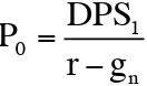
If you divide the left-hand side of the equation with EPS, that would be P/E! To continue, the right-hand side of the equation must be divided by the same EPS too. You would have the following equation:
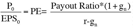
A market pricing of P/E can now be understood fundamentally on the underlying payout ratio, growth rate & cost of equity (and actually reinvestment rate too if you tweak further).
How do we use this?
When someone sells you a stock with a low P/E ratio, you ask the following questions to get more color:
What is the growth rate?
What is the dividend payout ratio (if there is)
What is the company’s cost of equity
How about for high-growth stock? Same testing methodology but instead of using a constant dividend model, you would use a 2-stage model of high growth and then add terminal value growth.
As long as you understand the concept above then the resultant formula below won’t be scary.
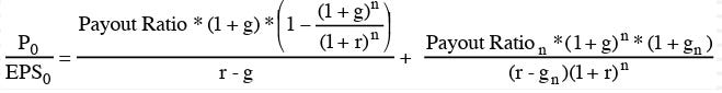
Understand and forget the formula above though we use the concept to understand more why P/E for some companies or industries are higher than the others.
Let’s test them out.
Consider you are asked to evaluate a high-growth company with the following characteristics; deconstructed between initial high-growth & later stable growth:
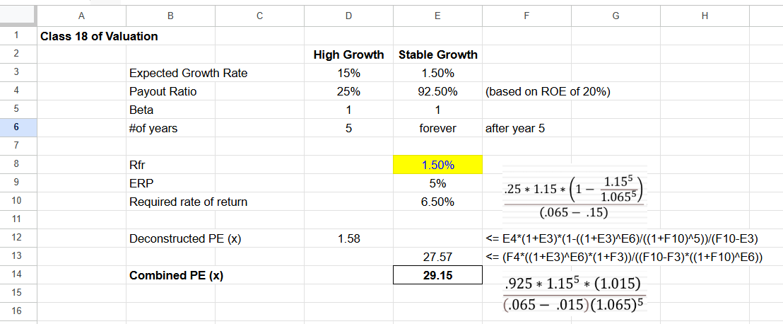
Risk-free rate is an important driver. To test it out, try changing from 1.5% to 4%.
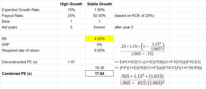
P/E immediately drops to 17.8x. [Link to the spreadsheet]
More on growth, risk-free rate, riskiness & ROE
Same goes with any adjustment to the expected growth rate. Prof did a data table on these 2 variables.
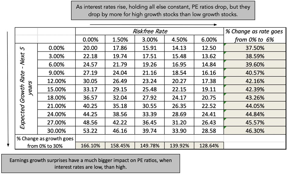
The above explains why P/E for stocks are high in previous years, due to ZIRP basically. In such ZIRP environment, the higher the growth, the higher the P/E. Thus, a growing company (that surpass estimates) has even higher P/E, in combo with lower cost of funding.
That “irrationality” in valuation is actually rationale; due to ZIRP.
The current decade where interest rates normalised, it becomes norm to actually expect lower earnings surprise.
Next, how do we identify superstar companies where growth is high while risk remains low? The drivers are on Low Beta & High Growth rates.
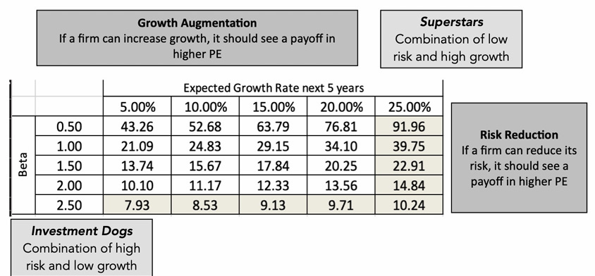
Be very careful when your screening criteria is only low P/E ratio. This would mean the lower left of the table above where stocks filtered have low growth and high beta (risk)!
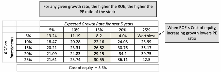
Growth must come with high ROI(C), not low ROI. This shows efficiency in reinvestment where the most growth you can get from lowest use in capital would give you higher P/E ratio.
Further test on low P/E ratio by country:
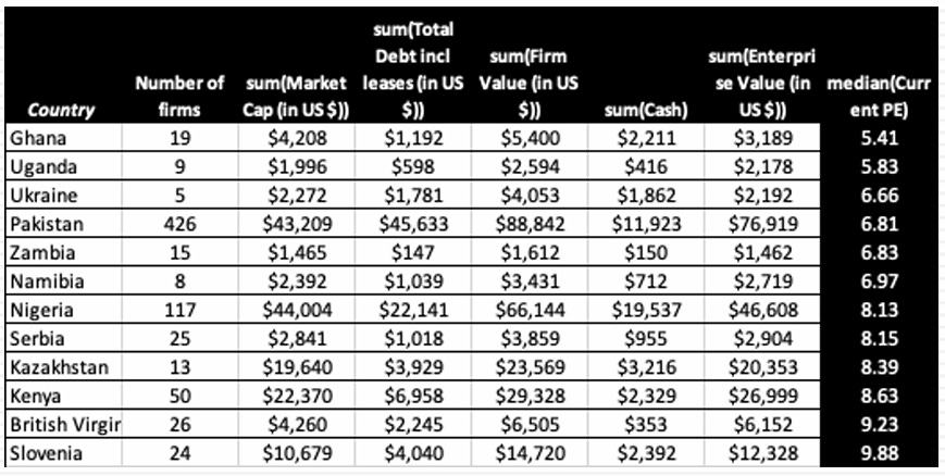
Countries above looked cheap because of high risk.
Let’s go further by evaluating the following mix bag of countries, which country would you choose to invest?
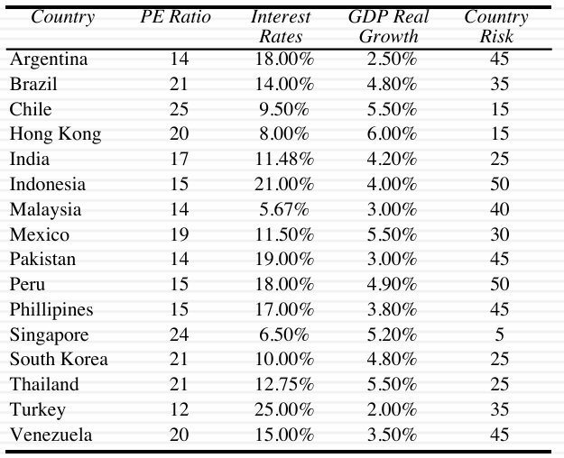
At first glance, it looks like they are fairly priced. A lowest P/E country like Turkey (12x) has higher interest rate (25%), country risk with a low GDP real growth (2%).
However, when putting the 3 drivers into a regression model. Some subtle differences arise.
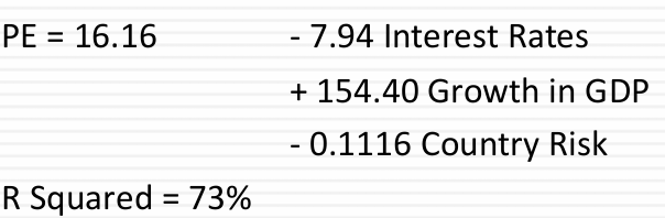
The equation shows (a very) positive correlation with GDP growth & inverse on rates & risk on a country P/E ratio. Plotting the 3 variables into this equation generates a Predicted PE for each country.
Sidetrack from a comment by Prof. Any regression that shows R-Squared of 90% are not worth evaluating because the relationship is obvious already. In financial regression, a 70% R-squared is as good as it gets.
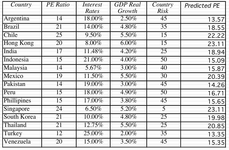
Though not by a big margin, we can see countries like HK, India, Malaysia plus a few more are priced lower that their predicted P/E (right column). While we would also avoid countries like Venezuela where their P/E is higher by a 5-point multiple.
More regression on equity and fixed-income yield
Using historical data to test if equity is expensive, an intermarket study too.
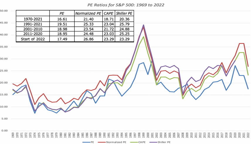
Based on the chart above, we can see that P/E ratio, by every means of calculating (Normalised, CAPE, Shiller) is declining in 2002/03. When compared by their periodic range in the table, a Normalised P/E of 26.86x seems expensive compared to previous decades.
Or is it actually cheap? Yes actually if you take interest rate into account using bond’s valuation.
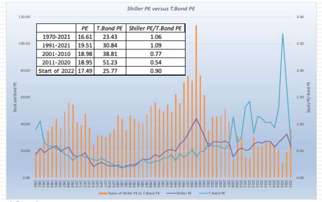
An equity P/E compared to a bond P/E (most sensitive to interest rate) is less than 1 since 2001. Thinking that S&P500 is expensive from P/E perspective as measured historically is wrong but should be measured against the prevailing interest rate.
A better comparison is to flip P/E into E/P, known as Earnings Yield. Like dividend yield, the higher it is, the “better/cheaper” for the company in generating the yield.
Predictability of Yield Curve (10y bond vs 2y bill yield)
Ever read that flat to negative yield curve is a predictor of incoming recession?
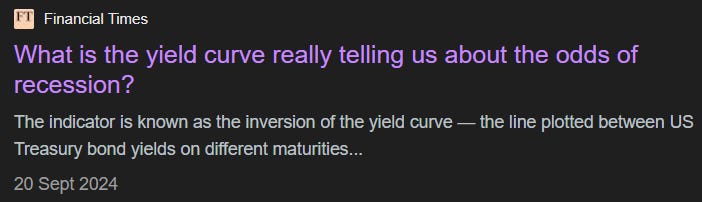
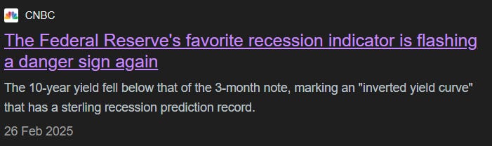

As of July 22, 2025, the yield for a 2-year U.S. government bond was ~4.38 percent, while the yield for a 10-year bond was ~3.88 percent. This represents an inverted yield curve, whereby bonds of longer maturities provide a lower yield, reflecting investors' expectations for a decline in long-term interest rates. Hence, making long-term debt holders open to more risk under the uncertainty around the condition of financial markets in the future.
Prof argues that this predictor is getting weaker post GFC as he runs through a correlation analysis. Hence, don’t need to pay so much attention on yield curve.
PEG Ratio
The PEG ratio is another test on driver of P/E, by testing the expected growth rate of companies. Essentially neutralising high growth vs low growth of companies.
However this is a flawed assumption as by dividing growth still don’t take away the embed growth in a P/E ratio.
The first formula below shows the deconstructed P/E that was shown above. The second formula divides both side by “growth”.
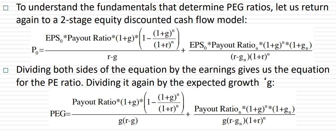
Growth is still embedded in the numerator.
Prof don’t agree with PEG ratios as growth is not linear as affected by difference in ROE & beta. A small PEG ratio company may still have the highest risk.
Book Value Multiples
Now let’s see if we can trust accountants to look at valuation! =)
Should we be excited if the stock is giving 0.5x Price/Book?
Let’s deconstructed again, this time ROE plays a big role.

A low ROE generally have low P/Bk. By definition, low ROE also have low cost of equity if the P/bk is ~1x.
Thus, a <1 P/bk generally means investors are expecting low ROIC (which also means low growth). There’s no arbitrage opportunity unless otherwise a full buyout or getting attention of activist investors.
EV/EBITDA
There’s an explosion of such use, compared to P/E because it fluctuates less overtime and has more data that has positive EBITDA versus negative Net Income.
A heavy capex company, or company in high re-investment rate stage will have high depreciation that would turn positive EBITDA from negative Net Income.
The only negative reason is that as a yardstick itself, the number is always lower than a P/E on the same company, making it look “cheap”.
For e.g. a company with EV/EBITDA of 5x has a P/E of 20x. A non-educated investor will think 5x EV/EBITDA is cheap but when presented a P/E of 20x, will think it is expensive. Same company.
Deconstructing EV/EBITDA:
Giving us the key drivers of:
Cost of Capital (not just Cost of Equity)
Expected growth rate
Tax rate
Re-investment rate
Tax rate is a key factor here compared to P/E which is already reflected in Net Income. EV/EBITDA uses pre-tax earnings. Meaning a higher tax rate would lower the EV/EBITDA. Thus, whenever a “good”, “low” EV/EBITDA is seen, especially compared against different countries is to ask, what is the tax rate for the companies.
When we do intrinsic valuation of getting EV from discounting FCF, the resulted EV can also be used to interpret by multiple of current EBITDA.
Price Enterprise/Revenue
Let’s go up further the P&L stack! By using just revenue, there’s virtually no company that cannot be benchmarked.
There’s 1 inconsistency across the board is that people unsure to use P/Revenue or EV/Revenue. By using P or Market Cap, you are basically ignoring the debt effect of a company. Hence best practice is to use EV/Revenue.
Without boring it with further deconstructed formula, the only key question to ask is what the margin of the company is. As always, a <1 EV/Revenue may seem low compared to a peer, but this company would also be having a lesser margin.
Value of Brand Name
When comes to margin, this is where a strong brand name comes in. The idea is to determine what is the value of a brand by comparing between 2 companies.
This is to dispel skeptics that says valuation don’t include branding, hence let’s add an arbitrary branding power in it. Double counting, overstating the valuation!
The effect of a strong brand name would just mean better pricing power, leading to better margin, which is always already reflected in the pricing multiple or DCF.
Using EV/Sales of a branded company versus a generic company, following is exactly how brand value is determined for when prof did such simulation many years back.
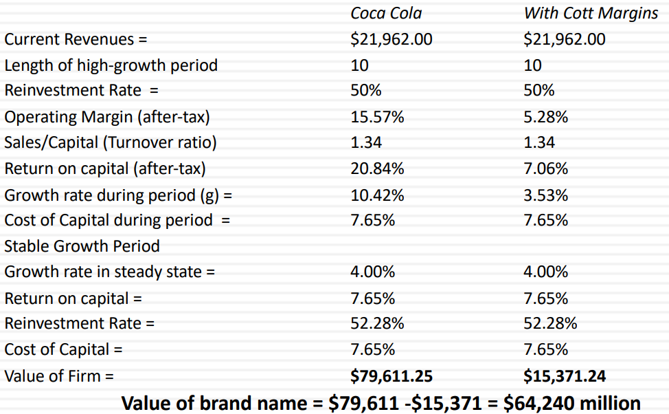
Prof did an intrinsic valuation of Coca-cola with the management ages ago. He derived that the intrinsic value was $79 billion. 1 of the folks objected the valuation saying that prof should add in another 20% premium to reflect the brand name of Coca-cola, because this is how they do it internally.
His reply? Because you do stupid things, doesn’t mean he has to!
The brand value is already embedded into the valuation, as seen in a higher margin.
Prof than contrast it with Cott, a Canadian generic coke. The numbers prove it. It has a lower margin, which reflects an eventual lower valuation of $15 billion.
If Coke management wants prof to add a premium on the brand than he should start with $15 billion and add a $64 billion premium so that it ends up as $79 billion.
Next, we’ll close the Pricing topic in transition via 2025’s syllabus before we move next to Private Companies Valuation. If adding/subtracting premium/discount arbitrary on items like “branding”, wait ‘till you see how this is abused in private companies.